The way I like to frame this problem deals with “covered” “grids”. A grid in this case is an n-by-n grid of unit squares, each of which can be colored or uncolored. An n-by-n grid is covered if each rectangle in the grid of area at least n contains a colored square. These images illustrate some examples!

This 4-by-4 grid is covered, as every rectangle in the grid of area at least 4 contains a colored square.

This 4-by-4 grid is not covered, as the red rectangle has an area of 4 and does not contain a colored square.

This 5-by-5 grid is not covered, as the red rectangle has an area of 6 (and thus an area greater than 5) and does not contain a colored square.

This 5-by-5 grid is covered, as every rectangle in the grid of area at least 5 contains a colored square.

Then, let T(n) be the minimum number of colored squares needed to cover an n-by-n grid.

We can see from the first and fourth examples that T(4) = 4 and T(5) = 5.

The main question I want to investigate is this: Does T(n) = O(n)? That is, is T(n) upper-bounded by some linear function in n?

We can easily see that T(n) is lower bounded by the function f(n) = n, since every row (and likewise column) must contain a colored square. But we can show that T(n) is strictly larger than this!

First, note that our example of a 4-by-4 grid that is covered by 4 colored squares is in fact the only example of a 4-by-4 that is covered by exactly 4 colored squares, up to the symmetries of a square.

To see this, first note that we require each row and column to have exactly one colored square, since otherwise the total number of colored squares would be greater than 4.

Then, using symmetry we can do a simple case bash, as described in the following images, to obtain this result.

By symmetry, we can just consider these three cases, as we will see that if we require a 4-by-4 grid has exactly 4 colored squares, these three configurations determine the entire grid.

In the first case, we see that the colored square in the second row is fully determined, as otherwise one of the two 2-by-2 squares will not contain a colored square. Likewise, the rest of the grid is also fully determined.

In the second case, we once again see that each colored square is fully determined. However, this results in there being a 2-by-2 square that does not contain a colored square, so this case fails.

Likewise, in the third case each colored square is fully determined, and this also results in there being a 2-by-2 square that does not contain a colored square. So we can finally conclude that the first case is the only possible case up to symmetry.

Next, note that for any n that is a multiple of 4, we can actually consider the first 4 rows of an n-by-n grid as being a 4-by-4 grid!

For example, in an 8-by-8 grid, if we look at the first 4 rows and group together the squares in 2-by-1 pairs, this forms a 4-by-4 grid. We can then consider one of these 2-by-1 pairs as being colored if at least one of the squares making up the pair is colored.

From this we see that if this 8-by-8 grid is covered, so is this embedded 4-by-4 grid!

Consider this 8-by-8 grid, which contains 10 colored squares and is in fact covered. We can then just focus on the first 4 rows.

Next, we can group together these squares into 2-by-1 rectangles, which we can then interpret as making up a 4-by-4 grid.

Then, we color each of these 2-by-1 rectangles if it contains a colored square, which results in this embedded 4-by-4 grid being covered, as expected.

Finally, if the first 4 rows of a covered 8-by-8 grid contain exactly 4 colored squares, up to symmetry each of these 2-by-1 rectangles contains a colored square.

Note that the above images generalize to any n-by-n grid for any n that is a multiple of 4.

Then, we have that the 3-by-m rectangles, where m is equal to the ceiling of n/3, must contain a colored square. This gives us a further restriction on the placement of colored squares in the first 4 rows of an n-by-n grid, assuming that there are exactly 4 colored squares in these first 4 rows.

We can then use this to show that this is impossible for n $>$ 4, as described in the following images.

As the ceiling of 8/3 is 3, we note that the 3-by-3 rectangles in the indicated corners must contain a colored square.

In the n = 8 case, we note that this uniquely determines the placement of the colored squares in the second and third row.

In general, we get that the horizontal distance between the colored squares in the second and third row must be greater than n minus 2 times the ceiling of n/3.

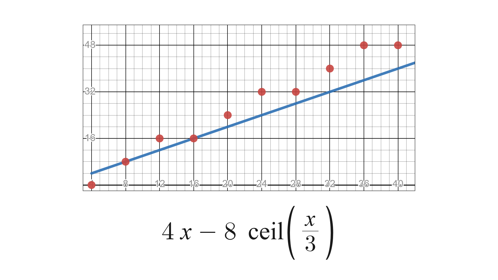
As such, this results in there being a rectangle that contains no colored squares with an area of 4 times n minus 8 times the ceiling of n/3. For n = 8, the resulting rectangle has an area of 8, so here our claim holds.

From all this, we see that, given an n a multiple of 4, to prove that the first 4 rows of a covered n-by-n grid must contain more than 4 colored squares, we can simply show that the area of this rectangle between the colored squares in the second and third rows must be greater than n for n $>$ 4.

We already have that this is true for n = 8, and the plot below shows that this does indeed hold true for n $>$ 4. So this implies that T(n) is greater than n for all multiples of 4 !

In fact, we do a lot better than just this! Note that the exact same argument applies to every consecutive 4 rows in an n-by-n grid, so we actually get that T(4n) is greater than or equal to 5n.

Furthermore, if we prove that T(k) = m, we get that T(kn) is greater than or equal to mn for all n, as we can perform a similar argument!

However, this alone is not enough to make progress towards whether T(n) is O(n) or not. This is as far as I got, but I’d wager that T(n) is not O(n).

One justification for this is that if T(n) was O(n), what constant could the limit of T(n)/n possibly be?

However, a better reason I think that T(n) is not O(n) is that this implies there are no Danzer sets in dimension 2 with a growth rate of O(r$^2$)!

https://en.wikipedia.org/wiki/Danzer_set

A Danzer set is a set of points in the plane such that every convex region of area 1 contains a point in this set. Such a set has a growth rate of O(r$^2$) if this set has a bounded density in the plane.

So given such a Danzer set with a density bounded by some real number k, we can scale an n-by-n grid by a factor of 1/sqrt(n) in each direction and center the grid at the origin.

Then, each rectangle in this grid that originally had an area greater than n now has an area greater than 1, and thus each of these rectangles contains at least one point in the Danzer set.

As such, we can then color each square that contains a point in this set, which must result in the grid being covered.

Finally, as the area of this scaled grid is n, the number of points will be less than kn, and thus so too will the number of colored squares.

Thus, given a Danzer set with bounded density, we obtain that T(n) is indeed O(n). But such a Danzer set existing also seems unlikely to me for similar reasons, and no one has found one yet.

This also means that if T(n) is not O(n), then no Danzer set of dimension 2 can have a bounded density! I wouldn’t bet on the converse holding though.

So this would solve that open problem, as well as a similar problem posed by Conway, called the dead fly problem! This was actually the original motivation for this problem, since I tried looking at a discrete version of this, which then ended up being implied by the original question!

Anyways, hope all this was interesting! This entire thread is also on an Overleaf file, so you can view it there at

https://www.overleaf.com/read/pdmjgyfthdzh

Have a good weekend everyone! :)